A Brief Introduction to Multilevel Models and Stan with R: rstanarm, brms, and rethinking
A Brief Introduction to Stan with R: rstanarm, brms, and rethinking
Overview
- Stan
- Probabilistic programming language written in C++
- Uses the No U-Turn Sampler (NUTS)
- Stan Interfaces
- Exist for R, python, julia, etc.
- Stan with R
Case Study: Multi-level Tadpoles
- Comes from Chapter 12 of (my favorite statistics) book Stastical Rethinking by Richard McElreath
- See the online lecture, which is part of his Winter 2019 class plus the slides
- More inspiration from McElreath’s blog post Multilevel Regression as Default
Code Sources
- Code for this case study is drawn primarily from two sources
- McElreath, Chapter 12 code
- Solomon Kurz, Chapter 12 code from his online book Statistical Rethinking with brms, ggplot2, and the tidyverse
- It goes through McElreath’s book doing the models using
brmsand thetidyverse
- It goes through McElreath’s book doing the models using
## install packages
pkgs <- c(
  "coda","mvtnorm","devtools","loo", # for rethinking
  'brms', 'rstanarm', 'rstan', 'tidyverse',
  'tidybayes', 'ggthemes', 'tictoc', 'ggstance',
  'bayesplot')
invisible(lapply(pkgs, function(x) {
  if(!require(x, character.only = TRUE)) install.packages(x)
}))

## install rethinking experimental branch
library(devtools)
devtools::install_github("rmcelreath/rethinking",ref="Experimental")
Example Part 1: Fixed Effects Model
Fixed vs Random (Pooling) Effects Models Refresher
- A robot visits a cafe and orders coffee in Paris…
- “Fixed Effects” models analagous to anmestic robot
- Forgets & overfits
- “Random Effects” models analagous to nmestic robot
- Remembers & regularizes
- “Fixed Effects” models analagous to anmestic robot
Un-pooled Model
Let’s get the reedfrogs data from rethinking.
## load rstan
library(rstan)
data('reedfrogs', package = 'rethinking')
d <- reedfrogs
rm('reedfrogs')
Making the tank cluster variable is easy. Keep as integer since Stan breaks if grouping variables are not integers.
d %>%
  head(10)
## density pred size surv propsurv
## 1 10 no big 9 0.9
## 2 10 no big 10 1.0
## 3 10 no big 7 0.7
## 4 10 no big 10 1.0
## 5 10 no small 9 0.9
## 6 10 no small 9 0.9
## 7 10 no small 10 1.0
## 8 10 no small 9 0.9
## 9 10 pred big 4 0.4
## 10 10 pred big 9 0.9d <- d %>%
dplyr::mutate(tank = 1:nrow(d))Here’s the formula for the un-pooled model in which each tank gets its own intercept (“fixed effects”).
\begin{align*}
\text{surv}_i        & \sim \text{Binomial} (n_i, p_i) \\
\text{logit} (p_i)   & = \alpha_{\text{tank}_i} \\
\alpha_{\text{tank}} & \sim \text{Normal} (0, 5)
\end{align*}
And \(n_i = \text{density}_i\). Now we’ll fit this simple aggregated binomial model (see Chapter 10 of Kurz or McElreath).
Building models with rethinking requires being explicit and specific about model parameters, emulating the way it is written out in mathematical notation.
rethinking
rethinking models interface with stan by translating the sytnax into Stan code, compiling, then sampling. We’ll me using the ulam function from the 2nd edition of the book. The 1st edition used map2stan which was more user friendly but had a less flexible syntax.
Stan breaks if you send more data than what is actually used by the model (declare_all_data = F option required to work)
tictoc::tic()
set.seed(12)
m12.1 <- rethinking::ulam(
    alist(
        surv ~ binomial( density , p ) ,
        logit(p) <- a_tank[tank] , # a_tank[tank] = "parameter a_tank grouped by [tank]"
        a_tank[tank] ~ normal( 0 , 5 )
    ),
    data = d,
    declare_all_data = FALSE, # only keep data used in model
    iter = 2000, warmup = 500, chains = 4, cores = 4)
tictoc::toc()
## 39.723 sec elapsedbrms
brms is similar to rethinking in that it translates the model to Stan code and compiles. The formula syntax, however, follows more traditional R formula model syntax, intentionally designed to emulate the formulate syntax of the popular lme4 package, which also fits Random Effects models but using flat priors and maximum likelihood (not bayes).
tictoc::tic()
b12.1 <-
  brms::brm(
    surv | trials(density) ~ 0 + factor(tank),
    data = d, family = binomial,
    prior = brms::prior(normal(0, 5), class = b),
    iter = 2000, warmup = 500, chains = 4, cores = 4,
    seed = 12)
tictoc::toc()
## 41.821 sec elapsedrstanarm
The same model but with rstanarm. Starts faster because it runs pre-complied Stan code. Has a formula syntax closer to that of lme4 and brms but requires specific functions calls to unlock the pre-compiled magic of the package. For example, if you want to run a simple linear model without random effects, then run stan_lm. If you want to run generalized linear models without random effects, then use stan_glm. For folks that use R, the suffixes _lm and _glm will be very familiar.
tictoc::tic()
a12.1 <-
  rstanarm::stan_glm(
    cbind(surv, density - surv) ~ 0 + as.factor(tank),
    data = d, family = binomial("logit"),
    prior = rstanarm::normal(0,5),
    iter = 2000, warmup = 500, chains = 4, cores = 4,
    seed = 12)
tictoc::toc()
## 3.833 sec elapsedCompare the model coefficient medians for the fixed effects model.
coef_m <- rethinking::coef(m12.1)
coef_b <- brms::fixef(b12.1)[,1]
coef_a <- coef(a12.1)
coef_mat <- cbind(coef_m, coef_b, coef_a) %>%
  'rownames<-'(sprintf('tank[%d]', 1:nrow(d))) %>%
  'colnames<-'(c('m', 'b', 'a'))
coef_mat
## m b a
## tank[1] 2.5279383336 2.49774103267 2.3577099423
## tank[2] 5.7418460838 5.69600186647 5.1810439261
## tank[3] 0.9151654134 0.91876402252 0.8997059529
## tank[4] 5.7436195973 5.72989907198 5.1938257147
## tank[5] 2.5163947670 2.49409442962 2.3455333998
## tank[6] 2.5068233213 2.52310988207 2.3803350233
## tank[7] 5.6829104358 5.72731048968 5.3542459949
## tank[8] 2.5279081858 2.52077155002 2.3876292416
## tank[9] -0.4307708896 -0.45496038928 -0.4356126228
## tank[10] 2.5120048175 2.50734795521 2.3650990199
## tank[11] 0.9333623570 0.93156514791 0.9039351204
## tank[12] 0.4288236135 0.44000579501 0.4301005974
## tank[13] 0.9176272606 0.92689685036 0.8884245986
## tank[14] -0.0071419376 0.00031940492 -0.0012609937
## tank[15] 2.5103163003 2.53349185853 2.3605923027
## tank[16] 2.5248295530 2.52915251349 2.3394564657
## tank[17] 3.4797111820 3.48583269244 3.3528230653
## tank[18] 2.5940997819 2.62512025339 2.5429584142
## tank[19] 2.1022544080 2.10429831011 2.0534638069
## tank[20] 6.3964811563 6.36851919816 5.8865138915
## tank[21] 2.6157010851 2.61793492017 2.5314236523
## tank[22] 2.6150352659 2.61070375916 2.5344384959
## tank[23] 2.6268295509 2.61523443682 2.5377702811
## tank[24] 1.7329273563 1.74292641493 1.7099431356
## tank[25] -1.2057007347 -1.19582377312 -1.1874387768
## tank[26] 0.0842104707 0.08729522189 0.0835779969
## tank[27] -1.7440567092 -1.73592867373 -1.7069571977
## tank[28] -0.5972061807 -0.59253703475 -0.5897240218
## tank[29] 0.0843675531 0.08673312089 0.0758520808
## tank[30] 1.4466307713 1.45254905507 1.4256110681
## tank[31] -0.7927095751 -0.77867327481 -0.7694869580
## tank[32] -0.4217235935 -0.42300963980 -0.4093781496
## tank[33] 3.8317083268 3.80086533156 3.6627959414
## tank[34] 2.9726508716 2.97066061469 2.8996971635
## tank[35] 2.9583434565 2.97727145398 2.8890364998
## tank[36] 2.1310176933 2.12846572290 2.0982976117
## tank[37] 2.1322857667 2.13845195527 2.1009623351
## tank[38] 6.6793997875 6.64843087462 6.1666916825
## tank[39] 2.9701961549 2.95816107240 2.9093906632
## tank[40] 2.4848070791 2.48288555381 2.4354791720
## tank[41] -2.1422040543 -2.13053194481 -2.0930368066
## tank[42] -0.6598561340 -0.66741801964 -0.6622635022
## tank[43] -0.5394615475 -0.54456101022 -0.5321473348
## tank[44] -0.4133118983 -0.41880814891 -0.4074381125
## tank[45] 0.5338648835 0.53785228404 0.5354522851
## tank[46] -0.6680192604 -0.66984404215 -0.6650005833
## tank[47] 2.1241553438 2.13245216673 2.1015544980
## tank[48] -0.0590177403 -0.05643394363 -0.0586473473Plotting Posterier Distributions of Coefficients
rethinking makes looking at coefficient estimates with varying affects easy. Add depth=2 because want to model within group.
# rethinking
rethinking::precis(m12.1, depth = 3) %>%
  rethinking::precis_plot()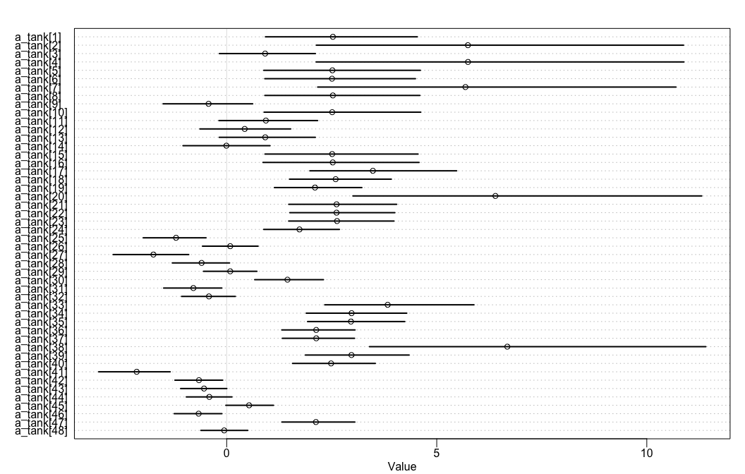
brms is a little tricker but we can use tidybayes to help make a similar coefficient plot.
# look at variable names
b12.1 %>%
  tidybayes::get_variables()
## [1] "b_factortank1" "b_factortank2" "b_factortank3" "b_factortank4"
## [5] "b_factortank5" "b_factortank6" "b_factortank7" "b_factortank8"
## [9] "b_factortank9" "b_factortank10" "b_factortank11" "b_factortank12"
## [13] "b_factortank13" "b_factortank14" "b_factortank15" "b_factortank16"
## [17] "b_factortank17" "b_factortank18" "b_factortank19" "b_factortank20"
## [21] "b_factortank21" "b_factortank22" "b_factortank23" "b_factortank24"
## [25] "b_factortank25" "b_factortank26" "b_factortank27" "b_factortank28"
## [29] "b_factortank29" "b_factortank30" "b_factortank31" "b_factortank32"
## [33] "b_factortank33" "b_factortank34" "b_factortank35" "b_factortank36"
## [37] "b_factortank37" "b_factortank38" "b_factortank39" "b_factortank40"
## [41] "b_factortank41" "b_factortank42" "b_factortank43" "b_factortank44"
## [45] "b_factortank45" "b_factortank46" "b_factortank47" "b_factortank48"
## [49] "lp__" "accept_stat__" "stepsize__" "treedepth__"
## [53] "n_leapfrog__" "divergent__" "energy__"b12.1 %>%
tidybayes::gather_draws(`b_factortank.*`, regex = TRUE) %>%
tidybayes::median_qi() %>%
ggplot2::ggplot(
ggplot2::aes(
y = .variable,
x = .value,
xmin = .lower,
xmax = .upper)) +
ggstance::geom_pointrangeh(position = ggstance::position_dodgev(height = .3))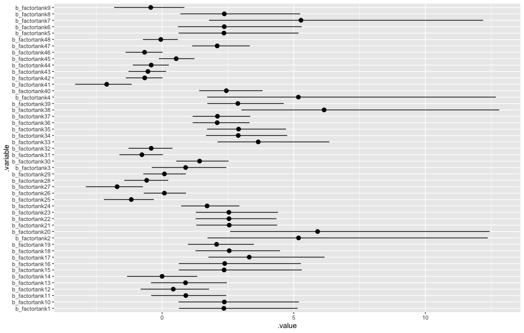
Finally, we can use bayesplot to plot results of an rstanarm object.
# look at variable names
posterior <- a12.1 %>%
  as.array()

pars <- dimnames(posterior)$parameters

bayesplot::color_scheme_set("gray")
posterior %>%
  bayesplot::mcmc_intervals(
    pars = pars)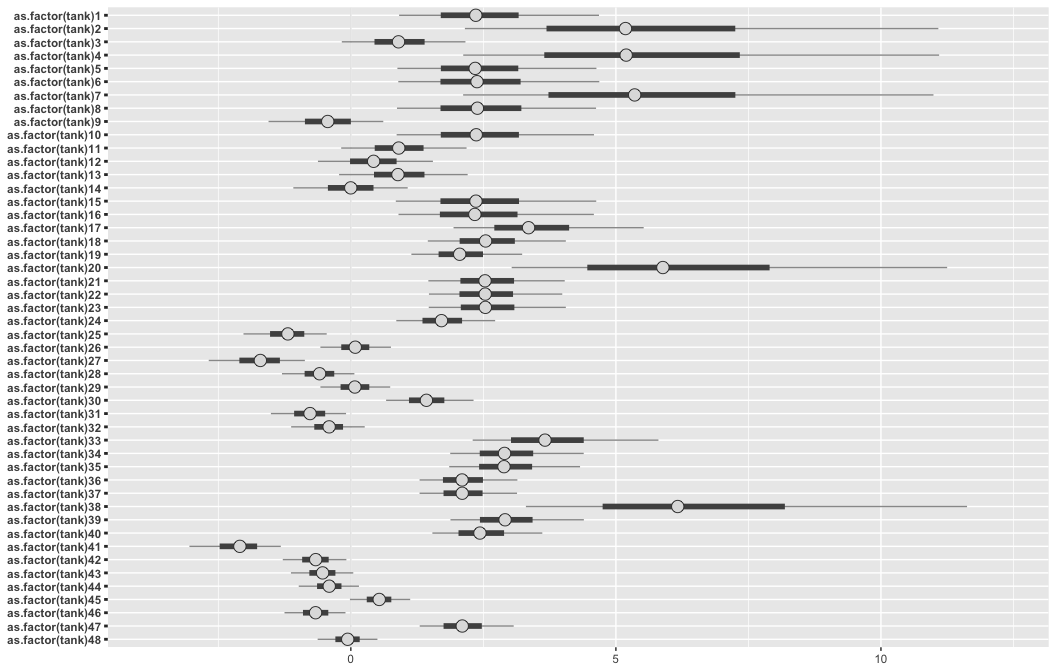
Multilevel Alternative aka “Pooling” aka “Random Effects”
The formula for the multilevel alternative is
\begin{align*}
\text{surv}_i        & \sim \text{Binomial} (n_i, p_i) \\
\text{logit} (p_i)   & = \alpha_{\text{tank}_i} \\
\alpha_{\text{tank}} & \sim \text{Normal} (\alpha, \sigma) \\
\alpha               & \sim \text{Normal} (0, 1) \\
\sigma               & \sim \text{HalfCauchy} (0, 1)
\end{align*}
rethinking random effects models are specified by assigning hyperparameters to original prior: a_tank[tank] ~ normal(0,5) becomes a_tank[tank] ~ normal(a, sigma) where a and sigma are the parameters for each tank’s intercepts. However, these parameters themselves have priors aka hyperpriors. This adds a second level to the model—hence, it is a multilevel model.
tictoc::tic()
set.seed(12)
m12.2 <-
  rethinking::ulam(
    alist(
        surv ~ binomial( density , p ) ,
        logit(p) <- a_tank[tank] ,
        # a_tank[tank] ~ normal( 0 , 5 ) , (before)
        a_tank[tank] ~ normal( a , sigma ) ,
        a ~ normal(0,1) , # hyperparameter for mean
        sigma ~ cauchy(0,1) # hyperparameter for group dispersion
    ),
    data=d, declare_all_data = FALSE,
    iter = 4000, warmup = 1000, chains = 4, cores = 4)
tictoc::toc()
## 34.935 sec elapsedHere is the same model using brms.
The syntax for the varying (random) effects follows the lme4 style, ( <varying parameter(s)> | <grouping variable(s)> ). In this case (1 | tank) indicates only the intercept, 1, varies by tank. The extent to which parameters vary is controlled by the prior, prior(cauchy(0, 1), class = sd), which is parameterized in the standard deviation metric. Do note that last part. It’s common in multilevel software to model in the variance metric, instead.
tictoc::tic()
b12.2 <-
  brms::brm(
    surv | trials(density) ~ 1 + (1 | tank),
    data = d, family = binomial,
    prior = c(brms::prior(normal(0, 1), class = Intercept),
              brms::prior(cauchy(0, 1), class = sd)),
    iter = 4000, warmup = 1000, chains = 4, cores = 4,
    seed = 12)
tictoc::toc()
## 35.742 sec elapsedrstanarm will again be very similar. However, note that are now using stan_glmer (note the er in glmer). This specifies that want to use a model with varying (random) effects. These models require that a grouping variable be specified i.e ( <varying parameter> | <grouping variable> ).
tictoc::tic()
a12.2 <-
  rstanarm::stan_glmer(
    cbind(surv, density - surv) ~ 1 + (1 | tank),
    data = d, family = binomial("logit"),
    prior_intercept = rstanarm::normal(0,1),
    prior = rstanarm::normal(0,1),
    iter = 4000, warmup = 1000, chains = 4, cores = 4,
    seed = 12)
tictoc::toc()
## 6.473 sec elapsed# extracting the coefficients is a little trickier with brms when using pooled models
coef_m <- rethinking::coef(m12.2)
# brms
coef_b <- c(coef(b12.2)$tank[,1,], brms::fixef(b12.2)[1], sd(brms::ranef(b12.2)$tank[,,1]))
# rstanarm
smry_a <- a12.2$stan_summary
coef_a <- c(coef(a12.2)$tank[,1], rstanarm::fixef(a12.2), smry_a[,'sd'][grepl('_NEW', names(smry_a[,'sd']))])
# woof, merge
coef_mat2 <- cbind(coef_m, coef_b, coef_a) %>%
'rownames<-'(c(sprintf('tank[%d]', 1:nrow(d)), 'a', 'sigma')) %>%
'colnames<-'(c('m', 'b', 'a'))
coef_mat2## m b a
## tank[1] 2.1232574871 2.1179248883 2.0766050111
## tank[2] 3.0518538063 3.0506456518 2.9459542719
## tank[3] 0.9926801392 0.9902473075 0.9624812207
## tank[4] 3.0456281868 3.0507013438 2.9550112913
## tank[5] 2.1153952972 2.1205965635 2.0629161508
## tank[6] 2.1346366450 2.1262561542 2.0680621683
## tank[7] 3.0547550205 3.0568624767 2.9473881804
## tank[8] 2.1201282632 2.1282739144 2.0766314787
## tank[9] -0.1792712587 -0.1856908109 -0.1811606611
## tank[10] 2.1170096279 2.1250090957 2.0629609349
## tank[11] 0.9914240942 0.9935635252 0.9704633234
## tank[12] 0.5734996537 0.5709686635 0.5613971684
## tank[13] 0.9948857927 0.9948499363 0.9683093073
## tank[14] 0.1994217655 0.1878940266 0.2018029427
## tank[15] 2.1306151864 2.1304523056 2.0723467221
## tank[16] 2.1368341432 2.1257254501 2.0595988662
## tank[17] 2.8944522357 2.9000015847 2.8293572939
## tank[18] 2.3882202784 2.3893754821 2.3537694089
## tank[19] 2.0034980197 2.0021628128 1.9745304244
## tank[20] 3.6612304325 3.6597771232 3.5494731747
## tank[21] 2.3898455014 2.3880652198 2.3430093053
## tank[22] 2.3909520451 2.3857416201 2.3444779124
## tank[23] 2.3873857353 2.3772498798 2.3463204305
## tank[24] 1.6998509692 1.6963075182 1.6818668229
## tank[25] -1.0005010124 -1.0090510217 -0.9947647185
## tank[26] 0.1603500731 0.1568512186 0.1586263761
## tank[27] -1.4285701827 -1.4382517265 -1.4138166690
## tank[28] -0.4770679730 -0.4745190424 -0.4722867023
## tank[29] 0.1593673173 0.1593301275 0.1467582922
## tank[30] 1.4410561032 1.4391074286 1.4250983144
## tank[31] -0.6360635684 -0.6411652349 -0.6341017501
## tank[32] -0.3083973541 -0.3122888467 -0.3144191408
## tank[33] 3.1742881596 3.1913875353 3.1110294571
## tank[34] 2.6985581578 2.7049312282 2.6584047520
## tank[35] 2.7012802460 2.7113443588 2.6520516735
## tank[36] 2.0658977032 2.0533977595 2.0276731653
## tank[37] 2.0544972783 2.0550000475 2.0333136913
## tank[38] 3.8799909179 3.8959472837 3.7881685622
## tank[39] 2.7055162518 2.6936471988 2.6616653516
## tank[40] 2.3498664405 2.3456441784 2.3058959917
## tank[41] -1.8111505869 -1.8180192259 -1.7947550803
## tank[42] -0.5815200680 -0.5740221341 -0.5691538767
## tank[43] -0.4512252565 -0.4564427957 -0.4525648339
## tank[44] -0.3402511174 -0.3390219202 -0.3376646426
## tank[45] 0.5776938530 0.5806971756 0.5685582711
## tank[46] -0.5743798160 -0.5752650289 -0.5731511192
## tank[47] 2.0546856021 2.0588911574 2.0276754612
## tank[48] 0.0039331294 -0.0010129768 0.0030743691
## a 1.2986202011 1.2839346906 1.2859972770
## sigma 1.6166030897 1.6514088432 1.6090644500Plotting: rethinking base R vs brms with ggplot2
Fig 12.1
Here’s base R code to reproduce Figure 12.1 of McElreath (2015).
The plot compares estimates of the multilevel model (open circles) with the that of the original empirical proportions (blue circles).
The multilevel model estimates exhibit shrinkage (regularization) towards the global proportion of survivors across all tanks.
## R code 12.5
# extract Stan samples
m_post <- rethinking::extract.samples(m12.2)

# compute median intercept for each tank
# also transform to probability with logistic
d$propsurv.est <- rethinking::logistic( apply( m_post$a_tank , 2 , median ) )

# display raw proportions surviving in each tank
plot( d$propsurv , ylim=c(0,1) , pch=16 , xaxt="n" ,
      xlab="tank" , ylab="proportion survival" , col=rethinking::rangi2,
      main    = "Multilevel shrinkage!")
axis( 1 , at=c(1,16,32,48) , labels=c(1,16,32,48) )

# overlay posterior medians
points( d$propsurv.est )

# mark posterior median probability across tanks
abline( h=rethinking::logistic(median(m_post$a)) , lty=2 )

# draw vertical dividers between tank densities
abline( v=16.5 , lwd=0.5 )
abline( v=32.5 , lwd=0.5 )
text( 8 , 0 , "small tanks" )
text( 16+8 , 0 , "medium tanks" )
text( 32+8 , 0 , "large tanks" )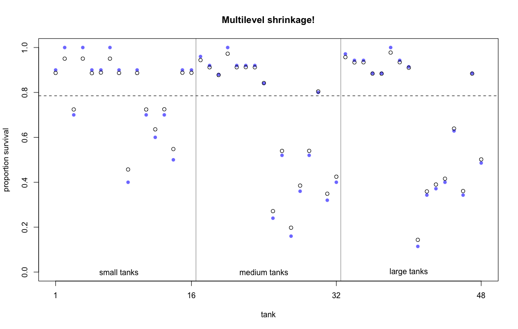
Here is a brms version using ggplot2 and ggthemes.
b_post <- brms::posterior_samples(b12.2, add_chain = T)

post_mdn <-
  coef(b12.2, robust = T)$tank[, , ] %>%
  dplyr::as_tibble() %>%
  dplyr::bind_cols(d) %>%
  dplyr::mutate(post_mdn = brms::inv_logit_scaled(Estimate))

post_mdn %>%
  ggplot2::ggplot(ggplot2::aes(x = tank)) +
  ggplot2::geom_hline(yintercept = brms::inv_logit_scaled(median(b_post$b_Intercept)), linetype = 2, size = 1/4) +
  ggplot2::geom_vline(xintercept = c(16.5, 32.5), size = 1/4) +
  ggplot2::geom_point(ggplot2::aes(y = propsurv), color = "orange2") +
  ggplot2::geom_point(ggplot2::aes(y = post_mdn), shape = 1) +
  ggplot2::coord_cartesian(ylim = c(0, 1)) +
  ggplot2::scale_x_continuous(breaks = c(1, 16, 32, 48)) +
  ggplot2::labs(title    = "Multilevel shrinkage!",
       subtitle = "The empirical proportions are in orange while the model-\nimplied proportions are the black circles. The dashed line is\nthe model-implied average survival proportion.") +
  ggplot2::annotate("text", x = c(8, 16 + 8, 32 + 8), y = 0,
           label = c("small tanks", "medium tanks", "large tanks")) +
  ggthemes::theme_fivethirtyeight() +
  ggplot2::theme(panel.grid = element_blank())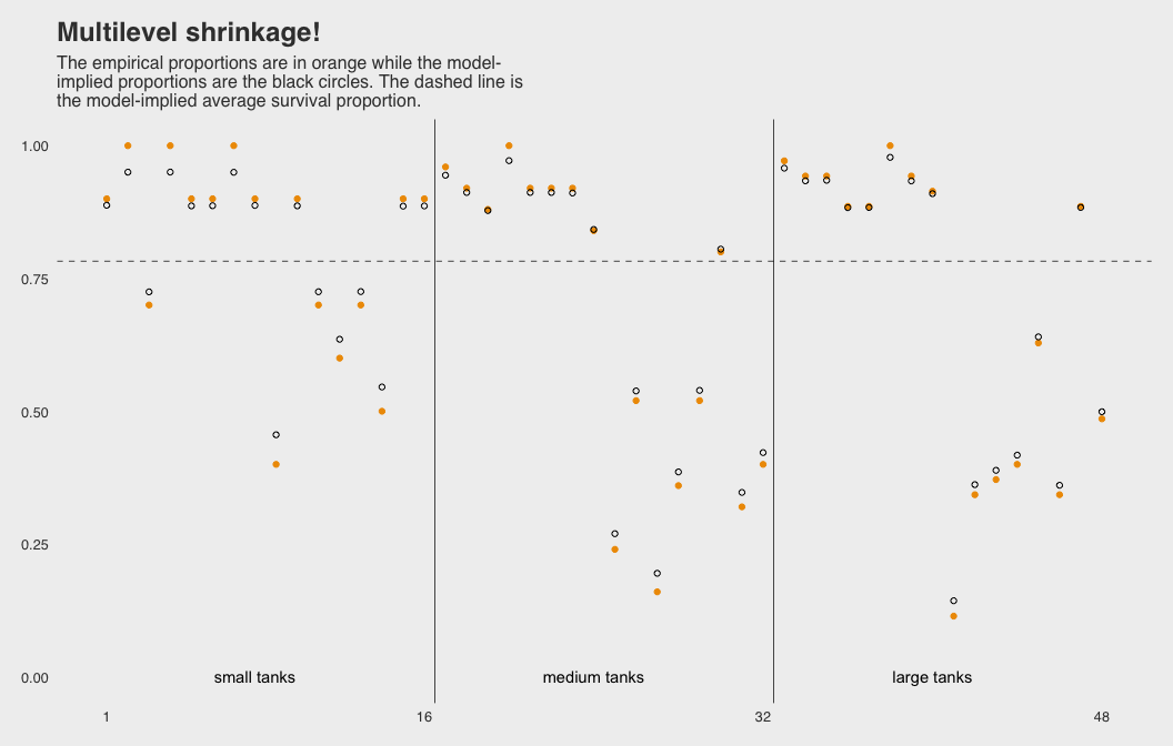
Fig 12.2.a
## R code 12.6
# show first 100 populations in the posterior
plot( NULL , xlim=c(-3,4) , ylim=c(0,0.35) ,
    xlab="log-odds survive" , ylab="Density" )
for ( i in 1:100 )
    curve( dnorm(x,m_post$a[i],m_post$sigma[i]) , add=TRUE ,
    col=rethinking::col.alpha("black",0.2) )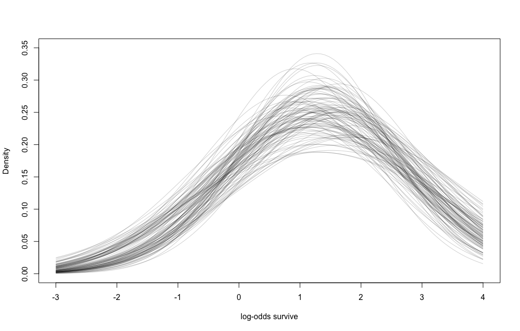
brms version of Figure 12.2.a
# this makes the output of `sample_n()` reproducible
set.seed(12)
b_post %>%
  dplyr::sample_n(100) %>%
  # keep chain and iter to differentiate iterations
  tidyr::expand(tidyr::nesting(iter, chain, b_Intercept, sd_tank__Intercept),
         x = seq(from = -4, to = 5, length.out = 100)) %>%
  dplyr::mutate(y = dnorm(x, b_Intercept, sd_tank__Intercept)) %>%
  ggplot2::ggplot() +
  ggplot2::geom_line(
    ggplot2::aes(x = x, y = y, group = paste(iter, chain)), # ensure unique iteration
            alpha = .2, color = "orange2") +
  ggplot2::labs(title = "Population survival distribution",
       subtitle = "The Gaussians are on the log-odds scale.") +
  ggplot2::scale_y_continuous(NULL, breaks = NULL) +
  ggplot2::coord_cartesian(xlim = c(-3, 4)) +
  ggthemes::theme_fivethirtyeight() +
  ggplot2::theme(
    plot.title    = ggplot2::element_text(size = 13),
    plot.subtitle = ggplot2::element_text(size = 10))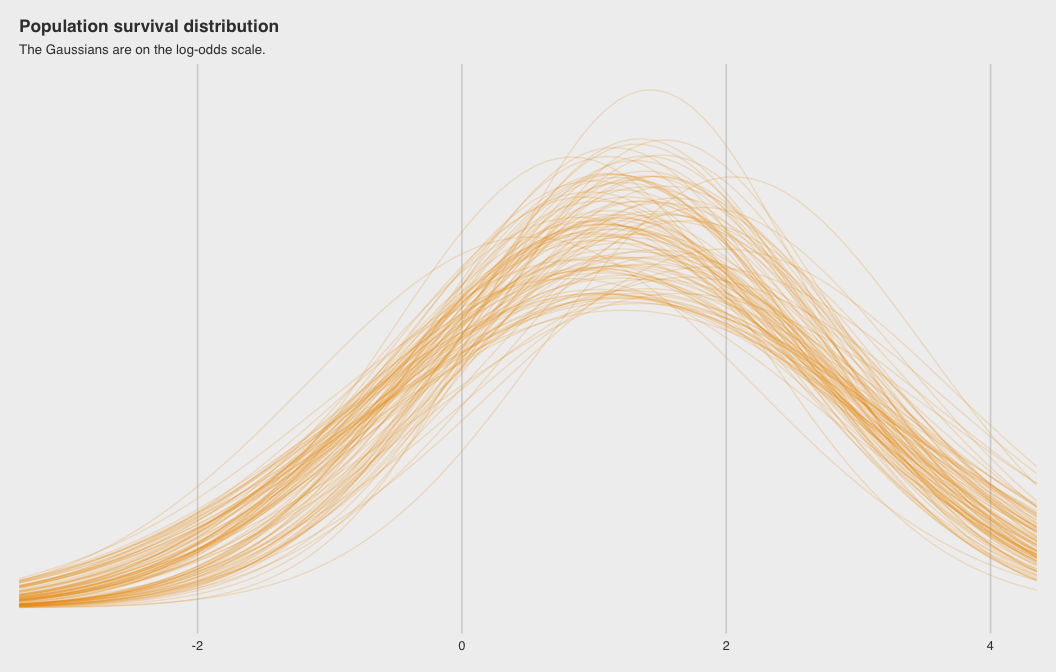
Note the uncertainty in terms of both location \(\alpha\) and scale \(\sigma\).
Fig 12.2.b
rethinking wrappers over base R to plot density curves of survival distribution.
# sample 12000 imaginary tanks from the posterior distribution
sim_tanks <- rnorm( 12000 , m_post$a , m_post$sigma )

# transform to probability and visualize
rethinking::dens(
  rethinking::logistic(sim_tanks),
  xlab="probability survive",
  main = "Population survival distribution")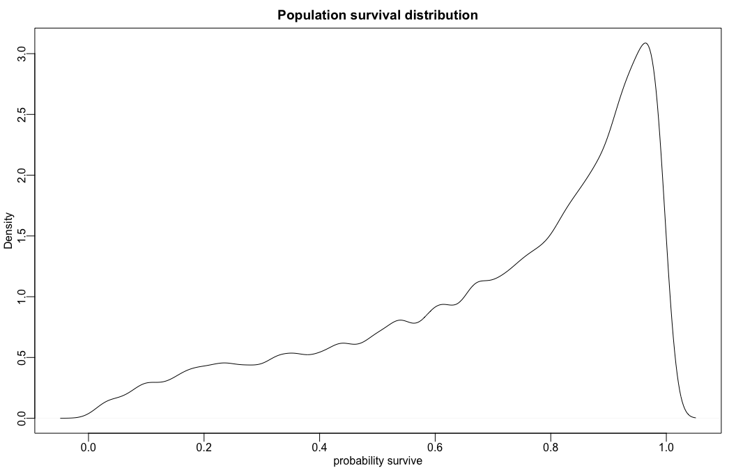
brms code
b_post %>%
  ggplot2::ggplot(
    ggplot2::aes(
      x =
        rnorm(
          n = nrow(b_post),
          mean = b_Intercept,
          sd   = sd_tank__Intercept) %>%
        brms::inv_logit_scaled(.))) +
    ggplot2::geom_density(size = 0, fill = "orange2") +
    ggplot2::scale_y_continuous(NULL, breaks = NULL) +
    ggplot2::ggtitle("Probability of survival") +
    ggthemes::theme_fivethirtyeight()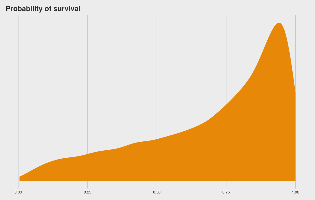
Other Bayesian (Stan) Resources
- Online Python book for the python folks out there
- Rasmus Bååth who has a nice course on Datacamp
- Michael Betancourt who has great case studies to learn from
- Stan Reference Manual is amazing